IQN model experiments

This page documents experiments on IQN model variants: use_ddqn (Double DQN), iqn_embedding_dimension, W_downsized / H_downsized (image dimensions), and related parameters.

How the runs relate (chain of changes):

• uni_12 → uni_16: only use_ddqn (False → True). Same: batch 512, speed 512, map 64–64, iqn_embedding_dimension 64, W/H 128.

• uni_16 → uni_17: only iqn_embedding_dimension (64 → 128). Same: use_ddqn True, batch/speed/map, W/H 128.

• uni_17 → uni_18: only W_downsized / H_downsized (128 → 256). Same: use_ddqn True, embedding 128, batch/speed/map.

• uni_17 → uni_19: W_downsized / H_downsized (128 → 64) and iqn_embedding_dimension (128 → 64). Same: use_ddqn True, batch/speed/map. “Downsized model” comparison.

• uni_17 → uni_20: only W_downsized / H_downsized (128 → 64). Same: iqn_embedding_dimension 128, use_ddqn True, batch/speed/map. Isolates image-size effect (embedding kept at 128).

So: uni_12 (baseline) → +DDQN → uni_16 → +embedding 128 → uni_17 → +image 256×256 → uni_18; also uni_17 → 64×64 + embedding 64 → uni_19; uni_17 → 64×64 (embedding 128) → uni_20. Each experiment below compares one pair; metrics are by relative time (and the analysis script also outputs by steps for equal gradient-update comparison).

Experiment 1: Double DQN (use_ddqn)

Experiment Overview

This experiment compared uni_16 (use_ddqn = True) with uni_12 (use_ddqn = False). All other settings (batch_size, running_speed, map cycle 64 hock – 64 A01, etc.) were the same so that the only change was the Q-learning variant.

Goal: Determine whether enabling Double DQN (1) improves overall race times and stability, and (2) shows the expected DDQN effect: reduced Q-value overestimation (targets computed with online network choosing the action, target network evaluating it).

What Double DQN does: With use_ddqn = True, the TD target uses the online network to select the best next action and the target network to evaluate it, instead of the target network doing both. This typically reduces overestimation of Q-values and can stabilize learning.

Results

Important: Run durations differed (uni_12 ~55 min, uni_16 ~70 min). All findings below are by relative time — minutes from run start; comparison uses the common window up to 55 min (when uni_12 ended).

Key findings:

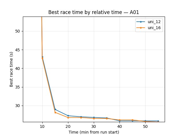
• Eval performance (trained_A01): uni_12 better — best time 24.850s vs 26.410s; finish rate at 55 min 50% vs 30%. So standard DQN-style (uni_12) gave better evaluation best time and higher eval finish rate in this window.

• Exploration (explo): uni_16 slightly better — at 55 min best 25.610s vs 25.890s, finish rate 53% vs 47%. DDQN (uni_16) had better exploration best time and higher explo finish rate.

• Hock: Slight edge to uni_16 — best at 55 min 61.440s vs 61.680s, finish rate 18% vs 17%.

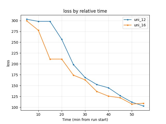
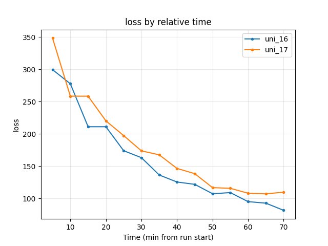
• Training loss: At 55 min uni_12 had lower loss (102.84 vs 109.16). In mid training (e.g. 20–45 min) uni_16 had lower loss (e.g. at 40 min 125.57 vs 144.92); by end of common window uni_12 was lower.

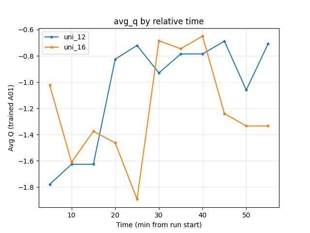
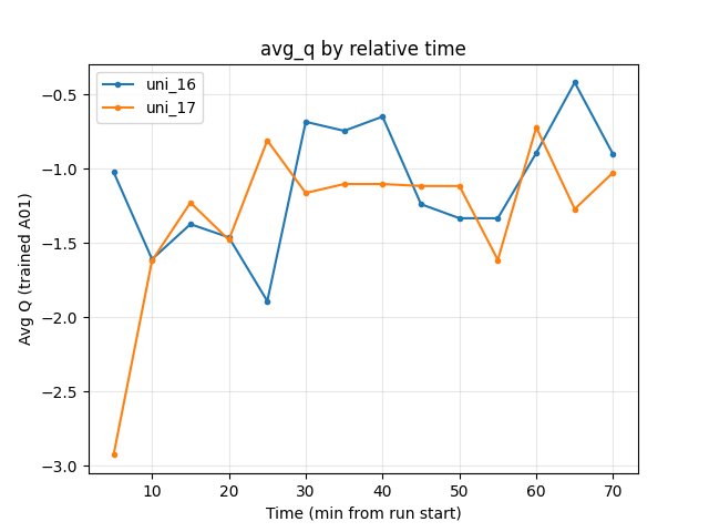
• Average Q (RL/avg_Q_trained_A01): At 55 min uni_12 -0.71, uni_16 -1.33. Uni_16 has more negative (lower) Q — consistent with reduced overestimation from Double DQN.

• GPU utilization: Both ~71–72%; no meaningful difference.

DDQN-specific takeaway: The lower average Q in uni_16 is what we would expect from Double DQN (less overestimation). There was no clear overall performance win: uni_12 was better on eval best time and eval finish rate; uni_16 was better on exploration finish rate and slightly better on explo/Hock best times. So we see the expected “less overestimation” signal from use_ddqn = True, but race-time results are mixed over 55 min.

Run Analysis

• uni_12: use_ddqn = False (standard DQN-style target), batch 512, speed 512, map cycle 64–64, ~55 min (relative time).

• uni_16: use_ddqn = True (Double DQN), same batch/speed/map cycle, ~70 min (relative time).

Comparison is over the common window up to 55 min.

Detailed TensorBoard Metrics Analysis

Methodology — Relative time (and by steps): Metrics are compared at checkpoints 5, 10, 15, 20, … 55 min; the same script also prints BY STEP tables (e.g. 50k, 100k steps) for equal-update comparison. Race times use per-race events (best/mean/std, finish rate); loss/Q/GPU use last value at that checkpoint. Source: python scripts/analyze_experiment_by_relative_time.py uni_12 uni_16 --interval 5 [--step_interval 50000]. The figures below show one metric per graph (runs as lines, by relative time).

trained_A01 — Eval (common window up to 55 min)

• Best time: uni_12 24.850s (from 20 min); uni_16 26.410s (from 40 min) → uni_12 better.

• Finish rate at 55 min: uni_12 50%, uni_16 30% → uni_12 better.

• Mean race time at 55 min: uni_12 164.49s, uni_16 218.53s (among finished+DNF) → uni_12 better.

trained_A01 — Explo (common window up to 55 min)

• Best time at 55 min: uni_12 25.890s, uni_16 25.610s → uni_16 slightly better.

• Finish rate at 55 min: uni_12 47%, uni_16 53% → uni_16 better.

trained_hock — Explo (common window up to 55 min)

• Best time at 55 min: uni_12 61.680s, uni_16 61.440s → uni_16 slightly better.

• Finish rate at 55 min: uni_12 17%, uni_16 18%.

Training Loss

• At 20 min: uni_12 256.84, uni_16 211.12.

• At 40 min: uni_12 144.92, uni_16 125.57 → uni_16 lower in mid training.

• At 55 min: uni_12 102.84, uni_16 109.16 → uni_12 lower at end of common window.

Average Q-values (RL/avg_Q_trained_A01)

• At 55 min: uni_12 -0.71, uni_16 -1.33 → uni_16 more negative. This is consistent with Double DQN reducing Q overestimation (lower, less optimistic Q).

GPU Utilization (Performance/learner_percentage_training)

• Both runs ~71–72% over the window; no significant difference.

Configuration Changes

Neural network (neural_network section in config YAML):

• uni_12: use_ddqn = False (target network both selects and evaluates next action).

• uni_16: use_ddqn = True (online network selects next action, target network evaluates it — Double DQN).

All other parameters (batch_size, running_speed, map cycle, etc.) matched between runs.

Hardware

• GPU: Same as uni_12 setup (see training_speed experiment).

• Parallel instances: 8 collectors.

• System: Same as other recent experiments.

Conclusions

• Overall: No clear “better” run over 55 min by relative time. uni_12 is better on eval (best time 24.85s, finish rate 50%). uni_16 is better on exploration (explo best time, explo finish rate, Hock best).

• Double DQN effect: uni_16 shows lower average Q (-1.33 vs -0.71 at 55 min), which is consistent with reduced Q overestimation from use_ddqn = True. So the intended effect of Double DQN (less overestimation) is visible; it did not translate into a clear eval win in this 55-minute window.

• Loss: DDQN had lower loss in mid training but slightly higher loss at 55 min; mixed.

Recommendations

• use_ddqn = True is reasonable if you care about less Q overestimation and possibly better exploration; in this experiment it did not improve eval best time or eval finish rate over 55 min.

• For eval-focused comparisons, standard DQN-style (use_ddqn = False) was better in this single comparison; more runs or longer runs would be needed to generalize.

• When comparing DDQN vs standard, always compare by relative time and report both race metrics (eval and explo) and Q / loss to separate “less overestimation” from “better policy”.

Experiment 2: iqn_embedding_dimension (128 vs 64)

Experiment Overview

This experiment compared uni_17 (iqn_embedding_dimension = 128) with uni_16 (iqn_embedding_dimension = 64). Both runs used use_ddqn = True and the same batch/speed/map cycle (64 hock – 64 A01).

Goal: See whether a larger quantile embedding dimension (more expressive return distribution) improves race times and stability, at the cost of extra parameters and compute.

Results

Important: Run durations differed (uni_16 ~70 min, uni_17 ~91 min). All findings are by relative time; comparison uses the common window up to 70 min.

Key findings:

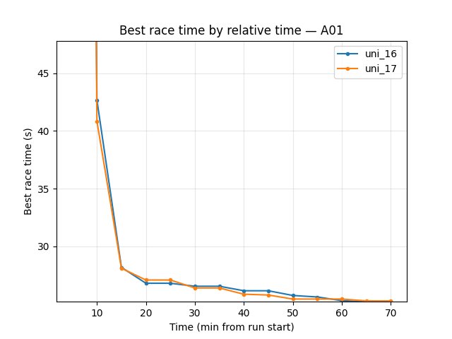
• Eval (trained_A01): uni_17 better — best time 24.71s–24.80s from 40 min onward; uni_16 reached 26.41s until 70 min when it hit 24.69s. Eval finish rate at 70 min: uni_17 52%, uni_16 36%. Larger embedding reached good eval times earlier and had higher eval finish rate.

• Explo (trained_A01): At 70 min best times close (uni_16 25.20s, uni_17 25.27s); finish rate uni_17 62% vs uni_16 59% — uni_17 slightly better on finish rate.

• Hock (explo): uni_16 better — at 70 min best 59.16s vs uni_17 62.30s; finish rate 24% vs 13%. Larger embedding worsened Hock in this window.

• Training loss: At 70 min uni_16 81.73, uni_17 109.87 → uni_16 lower (smaller embedding had lower loss by end of common window).

• Average Q: At 70 min uni_16 -0.90, uni_17 -1.03 — similar.

• GPU utilization: uni_17 slightly higher (~74–76%) vs uni_16 (~70–72%).

Takeaway: Larger iqn_embedding_dimension (128) improved A01 (eval best time, eval finish rate, explo finish rate) but hurt Hock (slower best time, lower finish rate) and increased loss. Trade-off: better short-track (A01), worse long track (Hock) over 70 min.

Run Analysis

• uni_16: iqn_embedding_dimension = 64, use_ddqn = True, ~70 min (relative time).

• uni_17: iqn_embedding_dimension = 128, use_ddqn = True, same other config, ~91 min (relative time).

Comparison is over the common window up to 70 min.

Detailed TensorBoard Metrics Analysis (uni_16 vs uni_17)

Methodology — Relative time (and by steps): Checkpoints 5, 10, … 70 min; script also outputs BY STEP tables. Source: python scripts/analyze_experiment_by_relative_time.py uni_16 uni_17 --interval 5 [--step_interval 50000].

trained_A01 — Eval (common window up to 70 min)

• Best time: uni_17 24.80s from 40 min, 24.71s at 65–70 min; uni_16 26.41s until 70 min when 24.69s → uni_17 reached good eval times earlier.

• Finish rate at 70 min: uni_16 36%, uni_17 52% → uni_17 better.

trained_A01 — Explo (common window up to 70 min)

• Best time at 70 min: uni_16 25.20s, uni_17 25.27s (close).

• Finish rate at 70 min: uni_16 59%, uni_17 62% → uni_17 slightly better.

trained_hock — Explo (common window up to 70 min)

• Best time at 70 min: uni_16 59.16s, uni_17 62.30s → uni_16 better (~3s faster).

• Finish rate at 70 min: uni_16 24%, uni_17 13% → uni_16 better.

Training Loss

• At 40 min: uni_16 125.57, uni_17 146.63.

• At 70 min: uni_16 81.73, uni_17 109.87 → uni_16 lower.

Average Q-values (RL/avg_Q_trained_A01)

• At 70 min: uni_16 -0.90, uni_17 -1.03 — similar.

GPU Utilization

• uni_16 ~70–72%; uni_17 ~74–76% over the window.

Configuration Changes (Experiment 2)

Neural network (neural_network section in config YAML):

• uni_16: iqn_embedding_dimension = 64.

• uni_17: iqn_embedding_dimension = 128.

All other parameters (use_ddqn = True, batch, speed, map cycle) matched.

Conclusions (Experiment 2)

• A01: Larger embedding (128) better — earlier and better eval best times, higher eval and explo finish rates over 70 min.

• Hock: Larger embedding worse — slower best time (62.30s vs 59.16s) and lower finish rate; uni_16 (64) clearly better on Hock.

• Loss: Smaller embedding (64) had lower loss at 70 min.

• Trade-off: iqn_embedding_dimension = 128 helps short track (A01) and hurts long track (Hock) in this comparison; more runs or longer runs would be needed to generalize.

Recommendations (Experiment 2)

• For A01-focused training, iqn_embedding_dimension = 128 may be worth trying; in this run it improved eval and explo on A01.

• For Hock / long maps, keeping 64 (or testing 128 with more data) is reasonable; 128 degraded Hock over 70 min.

• When comparing embedding sizes, compare by relative time and report both A01 and Hock (or all maps) to see the trade-off.

Experiment 3: Image dimensions (W_downsized / H_downsized 256 vs 128)

Experiment Overview

This experiment compared uni_18 (W_downsized = 256, H_downsized = 256) with uni_17 (W_downsized = 128, H_downsized = 128). Both runs used the same IQN settings (iqn_embedding_dimension = 128, use_ddqn = True) and batch/speed/map cycle (64 hock – 64 A01).

Goal: See whether larger input images (256×256 vs 128×128) improve race times and stability at the cost of more CNN compute and memory.

Results

Important: Run durations differed (uni_17 ~91 min, uni_18 ~146 min). All findings are by relative time; comparison uses the common window up to 90 min.

Key findings:

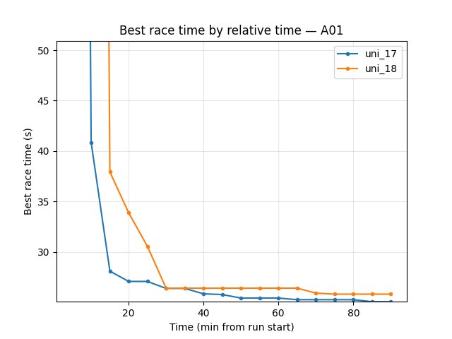
• Eval (trained_A01): By 90 min best time is close — uni_17 24.71s, uni_18 24.70s (uni_18 slightly better). Finish rate at 90 min: uni_17 59%, uni_18 44% → uni_17 better. uni_18 reached first eval finish much later (first finish ~32 min vs ~7.6 min for uni_17); slower convergence with 256×256.

• Explo (trained_A01): uni_17 better — at 90 min best 25.07s vs uni_18 25.82s; finish rate 68% vs 53%.

• Hock (explo): uni_17 better — at 90 min best 58.60s vs uni_18 61.29s (~2.7s faster); finish rate 19% vs 15%.

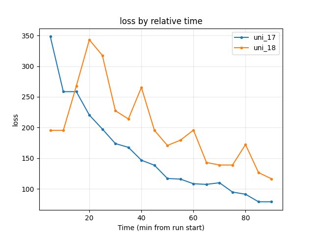
• Training loss: At 90 min uni_17 78.86, uni_18 116.27 → uni_17 lower.

• Average Q: At 90 min uni_17 -0.74, uni_18 -0.86 — similar.

• GPU utilization: uni_17 ~73–76%; uni_18 ~89–90% — 256×256 uses much more GPU (larger CNN), so more compute per step and potentially slower throughput.

Takeaway: Larger image (256×256) in uni_18 led to slower convergence (later first finishes, lower finish rates over 90 min), worse explo best times and Hock (61.29s vs 58.60s), and higher loss. Only a marginal gain on eval best A01 (24.70s vs 24.71s) by 90 min. Over the 90-minute common window, 128×128 (uni_17) is better on most metrics; 256×256 did not pay off in this run.

Run Analysis

• uni_17: W_downsized = 128, H_downsized = 128, iqn_embedding_dimension = 128, use_ddqn = True, ~91 min (relative time).

• uni_18: W_downsized = 256, H_downsized = 256, same IQN/batch/speed/map cycle, ~146 min (relative time).

Comparison is over the common window up to 90 min.

Detailed TensorBoard Metrics Analysis (uni_17 vs uni_18)

Methodology — Relative time (and by steps): Checkpoints 5, 10, … 90 min; script also outputs BY STEP tables. Source: python scripts/analyze_experiment_by_relative_time.py uni_17 uni_18 --interval 5 [--step_interval 50000].

trained_A01 — Eval (common window up to 90 min)

• Best time at 90 min: uni_17 24.71s, uni_18 24.70s (close; uni_18 marginally better).

• Finish rate at 90 min: uni_17 59%, uni_18 44% → uni_17 better.

• First finish: uni_17 ~7.6 min, uni_18 ~32.2 min → uni_17 converged much earlier.

trained_A01 — Explo (common window up to 90 min)

• Best time at 90 min: uni_17 25.07s, uni_18 25.82s → uni_17 better.

• Finish rate at 90 min: uni_17 68%, uni_18 53% → uni_17 better.

trained_hock — Explo (common window up to 90 min)

• Best time at 90 min: uni_17 58.60s, uni_18 61.29s → uni_17 better (~2.7s faster).

• Finish rate at 90 min: uni_17 19%, uni_18 15%.

Training Loss

• At 85 min: uni_17 78.84, uni_18 126.49.

• At 90 min: uni_17 78.86, uni_18 116.27 → uni_17 lower.

Average Q-values (RL/avg_Q_trained_A01)

• At 90 min: uni_17 -0.74, uni_18 -0.86 — similar.

GPU Utilization (Performance/learner_percentage_training)

• uni_17 ~73–76% over the window; uni_18 ~89–90% — uni_18 uses much more GPU (4× pixels, larger CNN).

Configuration Changes (Experiment 3)

Neural network (neural_network section in config YAML):

• uni_17: W_downsized = 128, H_downsized = 128.

• uni_18: W_downsized = 256, H_downsized = 256.

All other parameters (iqn_embedding_dimension = 128, use_ddqn = True, batch, speed, map cycle) matched.

Conclusions (Experiment 3)

• Convergence: 256×256 (uni_18) slower — first eval finish ~32 min vs ~7.6 min for 128×128 (uni_17).

• Eval best time: By 90 min nearly tied (24.70s vs 24.71s); eval finish rate and explo/Hock clearly better for 128×128.

• Loss: 128×128 had lower loss at 90 min.

• GPU: 256×256 raised GPU use to ~90% vs ~74%; more compute per step did not yield better policy over 90 min.

• Recommendation: 128×128 is better in this 90-minute window; 256×256 did not pay off.

Recommendations (Experiment 3)

• Keep W_downsized / H_downsized = 128 for this setup unless longer runs or different maps show a clear gain for 256×256.

• If trying 256×256 again, compare by relative time over a long common window and report finish rates and Hock as well as eval best time; expect higher GPU use and slower convergence early.

Interpretation and literature (Experiment 3)

The following are plausible interpretations from the literature; they are not proven for this specific setup but help frame the 256×256 vs 128×128 results.

1. Is the worse performance because the larger model simply learns slower?

• Partly plausible. In DRL, larger networks (more parameters, higher-resolution inputs) often need more gradient steps and more data to reach the same performance; optimal learning rate also tends to decrease with longer training. Over a fixed 90-minute wall-clock window, the 256×256 run does fewer effective updates per minute (higher GPU use per step), so it is both “slower per step” and “fewer steps in the same time.” So slower learning in wall-clock time is a reasonable part of the explanation.

• Literature: scaling surveys suggest longer training and tuned learning-rate scaling for larger models; see e.g. “Scaling DRL for Decision Making” (data, network, and training budget) and work on learning-rate scaling with model/training size.

2. Or is it because the model is not just bigger but excessively big (memorizing instead of generalizing)?

• Possible but harder to separate here. In supervised settings, excess capacity can lead to memorization and worse generalization; in DRL the picture is mixed — some work reports that naively increasing capacity in DRL often hurts (instability, no gain) rather than improving. Vision-based RL with higher resolution also increases the risk of confounding visual factors and overfitting to training tracks. In this experiment we did not test on unseen maps; worse finish rates and Hock for 256×256 could reflect either slower learning or worse generalization (e.g. overfitting to A01). So “excess capacity / memorization” is a plausible contributing factor but not distinguishable from “just slower” in this single comparison.

• Literature: “Training Larger Networks for Deep Reinforcement Learning” (Ota et al., arXiv:2102.07920) shows that naively scaling network size in DRL does not improve performance and can cause instability; successful scaling in that work required architectural and training changes (wider DenseNet-like connections, decoupling representation learning, distributed training to reduce overfitting).

3. What might need to be tuned to train the larger (256×256) model properly?

• Likely candidates (from literature and practice): - Longer training: Compare 256×256 vs 128×128 at equal number of gradient steps or equal environment steps, not only equal wall-clock time; and/or run 256×256 for much longer (e.g. 2×–3×) to see if it eventually matches or surpasses 128×128. - Learning rate: Larger models often need different (often smaller) learning rates; try a lower learning rate for the 256×256 setup, or use a schedule that keeps LR lower in the second half of training. - Batch size / replay: Larger batches or more replay can stabilize training for larger networks; if GPU memory allows, try a larger batch size for 256×256 so that each update uses more data. - Architecture and training recipe: Ota et al. (arXiv:2102.07920) argue that wider networks with skip (DenseNet-like) connections, decoupling representation learning from RL (e.g. pretrain or separately train the CNN), and distributed / multi-GPU training to mitigate overfitting are important for scaling DRL. Our setup uses a single CNN trained end-to-end; adding representation decoupling or different connectivity could help 256×256. - Regularization: Slightly stronger regularization (e.g. weight decay, dropout in the CNN) might help if the larger model is overfitting.

Summary: The 90-minute results are consistent with slower learning in wall-clock time for 256×256 (fewer updates, same hyperparameters). Excess capacity / memorization is a possible additional factor but not verified here. To give 256×256 a fair chance, try longer runs, learning-rate and batch-size tuning, and optionally architectural / representation-learning changes as in the “Training Larger Networks for Deep RL” line of work.

Experiment 4: Image dimensions 64×64 vs 128×128 (downsized model)

Experiment Overview

This experiment compared uni_19 (W_downsized = 64, H_downsized = 64, iqn_embedding_dimension = 64) with uni_17 (W_downsized = 128, H_downsized = 128, iqn_embedding_dimension = 128). Both runs used use_ddqn = True and the same batch/speed/map cycle (64 hock – 64 A01).

Goal: See whether a downsized model (smaller images and smaller embedding) can match or improve race times while reducing GPU compute, or whether the lower resolution hurts performance.

Note: uni_19 differs in two parameters — image size (64×64 vs 128×128) and embedding (64 vs 128) — so this is a “downsized model” comparison rather than an isolated image-size test.

Results

Important: Run durations differed (uni_17 ~91 min, uni_19 ~150 min). All findings are by relative time; comparison uses the common window up to 90 min.

Key findings:

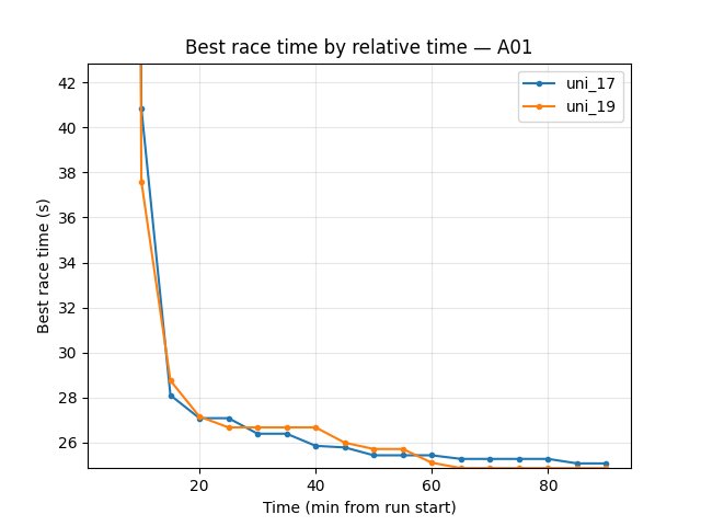
• Eval (trained_A01): uni_17 better — best time at 90 min 24.71s vs 24.95s; finish rate 59% vs 47%; first eval finish ~7.6 min vs ~23.5 min. uni_17 converged much earlier and had better eval best time and finish rate.

• Explo (trained_A01): uni_19 better on best time — at 90 min 24.86s vs 25.07s (~0.2s faster); finish rate uni_17 68% vs uni_19 64% (close). So 64×64 reached a slightly better explo best A01 time by 90 min.

• Hock (explo): uni_17 much better — at 90 min best 58.60s vs uni_19 65.52s (~7s faster); finish rate 19% vs 3%. Early in training (5–45 min), uni_19 had better Hock times (e.g. 67.23s vs 64.33s at 45 min); uni_17 overtook and pulled ahead by 90 min.

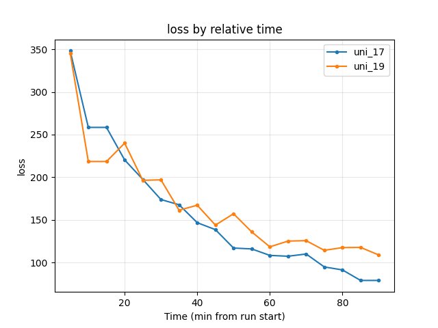
• Training loss: At 90 min uni_17 78.86, uni_19 108.72 → uni_17 lower.

• Average Q: At 90 min uni_17 -0.74, uni_19 -1.09 — similar.

• GPU utilization: uni_17 ~73–76%; uni_19 ~66–69% — 64×64 uses less GPU (smaller CNN and embedding).

Takeaway: The downsized model (64×64, embedding 64) reached a slightly better explo A01 best time by 90 min and used less GPU, but had slower convergence (later first eval finish), lower eval finish rate, and much worse Hock (best time 65.52s vs 58.60s). Trade-off: lower compute and marginally better explo A01 best vs worse eval and Hock.

Run Analysis

• uni_17: W_downsized = 128, H_downsized = 128, iqn_embedding_dimension = 128, use_ddqn = True, ~91 min (relative time).

• uni_19: W_downsized = 64, H_downsized = 64, iqn_embedding_dimension = 64, use_ddqn = True, same batch/speed/map cycle, ~150 min (relative time).

Comparison is over the common window up to 90 min.

Detailed TensorBoard Metrics Analysis (uni_17 vs uni_19)

Methodology — Relative time (and by steps): Checkpoints 5, 10, … 90 min; script also outputs BY STEP tables. Source: python scripts/analyze_experiment_by_relative_time.py uni_17 uni_19 --interval 5 [--step_interval 50000].

trained_A01 — Eval (common window up to 90 min)

• Best time at 90 min: uni_17 24.71s, uni_19 24.95s → uni_17 better.

• Finish rate at 90 min: uni_17 59%, uni_19 47% → uni_17 better.

• First finish: uni_17 ~7.6 min, uni_19 ~23.5 min → uni_17 converged much earlier.

trained_A01 — Explo (common window up to 90 min)

• Best time at 90 min: uni_17 25.07s, uni_19 24.86s → uni_19 better (~0.2s faster).

• Finish rate at 90 min: uni_17 68%, uni_19 64% (close).

trained_hock — Explo (common window up to 90 min)

• Best time at 90 min: uni_17 58.60s, uni_19 65.52s → uni_17 better (~7s faster).

• Finish rate at 90 min: uni_17 19%, uni_19 3%.

• Early on (5–45 min): uni_19 had better Hock (67.23s, 67.47s) vs uni_17 (72.16s down to 64.33s); uni_17 overtook by ~50 min.

Training Loss

• At 90 min: uni_17 78.86, uni_19 108.72 → uni_17 lower.

Average Q-values (RL/avg_Q_trained_A01)

• At 90 min: uni_17 -0.74, uni_19 -1.09 — similar.

GPU Utilization (Performance/learner_percentage_training)

• uni_17 ~73–76%; uni_19 ~66–69% over the window — uni_19 uses less GPU.

By steps (common step window up to 3.3M steps)

• Eval best A01 at 3.3M steps: uni_17 24.71s, uni_19 24.95s (uni_19 reached this at ~3M steps).

• Explo best A01 at 3.3M steps: uni_17 25.05s, uni_19 24.86s → uni_19 better.

• Hock best at 3.3M steps: uni_17 58.60s, uni_19 65.52s → uni_17 better.

• Loss at 3.3M steps: uni_17 75.87, uni_19 117.59 → uni_17 lower.

Configuration Changes (Experiment 4)

Neural network (neural_network section in config YAML):

• uni_17: W_downsized = 128, H_downsized = 128, iqn_embedding_dimension = 128.

• uni_19: W_downsized = 64, H_downsized = 64, iqn_embedding_dimension = 64.

All other parameters (use_ddqn = True, batch, speed, map cycle) matched.

Conclusions (Experiment 4)

• Eval: 64×64 (uni_19) slower convergence (first eval finish ~23.5 min vs ~7.6 min) and worse best time and finish rate at 90 min.

• Explo A01: 64×64 reached slightly better best explo A01 (24.86s vs 25.07s) by 90 min; finish rates similar.

• Hock: 64×64 much worse — best 65.52s vs 58.60s, finish rate 3% vs 19%.

• GPU: 64×64 uses less GPU (~67% vs ~74%).

• Loss: 128×128 had lower loss at 90 min.

• Trade-off: 64×64 reduces compute and can match or slightly beat explo A01 best time, but at the cost of slower convergence, worse eval, and much worse Hock.

Recommendations (Experiment 4)

• Keep 128×128 for balanced performance across eval, explo, and Hock unless GPU is severely constrained.

• 64×64 is viable if you prioritize A01-only training or lower GPU usage and can accept worse Hock and slower eval convergence.

• For Hock / long maps, 64×64 with embedding 64 is not recommended; see Experiment 5 for 64×64 with embedding 128 (much better Hock).

Experiment 5: Image dimensions 64×64 vs 128×128 (embedding 128 — isolates resolution)

Experiment Overview

This experiment compared uni_20 (W_downsized = 64, H_downsized = 64, iqn_embedding_dimension = 128) with uni_17 (W_downsized = 128, H_downsized = 128, iqn_embedding_dimension = 128). Both runs used use_ddqn = True and the same batch/speed/map cycle (64 hock – 64 A01).

Goal: Isolate the effect of image resolution by keeping embedding at 128. This answers whether the poor Hock performance in uni_19 (64×64, embedding 64) was caused by lower resolution or by the smaller embedding.

Note: Only image size differs — embedding is 128 in both. This is the clean image-resolution comparison.

Results

Important: Run durations differed (uni_17 ~91 min, uni_20 ~120 min). All findings are by relative time; comparison uses the common window up to 90 min.

Key findings:

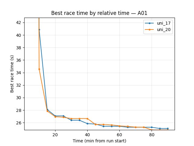
• Eval (trained_A01): uni_20 better — best time at 90 min 24.72s vs 24.71s (tied); finish rate 70% vs 59%; first eval finish ~15.5 min vs ~7.6 min (uni_17 converged earlier, but uni_20 reached higher finish rate by 90 min).

• Explo (trained_A01): uni_20 better — at 90 min best 24.84s vs 25.07s (~0.23s faster); finish rate 67% vs 68% (similar).

• Hock (explo): uni_17 slightly better — at 90 min best 58.60s vs uni_20 59.09s (~0.5s gap). Finish rate uni_20 23% vs uni_17 19% — uni_20 better on finish rate. The Hock gap is much smaller than in uni_19 (65.52s) vs uni_17 (58.60s), confirming that the ~7s deficit in uni_19 came from embedding 64, not image resolution.

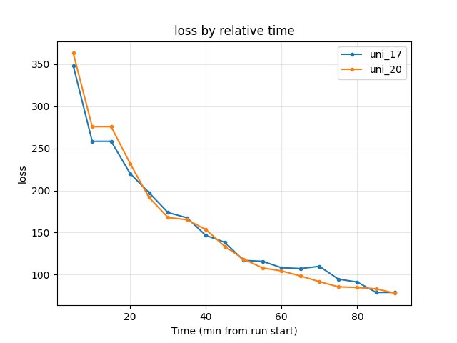
• Training loss: At 90 min uni_17 78.86, uni_20 77.84 → uni_20 lower.

• Average Q: At 90 min similar (uni_17 -0.74, uni_20 -1.26).

• GPU utilization: uni_17 ~73–76%; uni_20 ~66–67% — 64×64 uses less GPU.

Takeaway: 64×64 with embedding 128 (uni_20) is competitive with 128×128 (uni_17). It matches or beats on eval finish rate, explo best A01, and loss; uses less GPU; Hock is only ~0.5s slower vs ~7s in uni_19. Conclusion: the poor Hock in uni_19 was due to embedding 64, not image resolution.

Run Analysis

• uni_17: W_downsized = 128, H_downsized = 128, iqn_embedding_dimension = 128, use_ddqn = True, ~91 min (relative time).

• uni_20: W_downsized = 64, H_downsized = 64, iqn_embedding_dimension = 128, use_ddqn = True, same batch/speed/map cycle, ~120 min (relative time).

Comparison is over the common window up to 90 min.

Detailed TensorBoard Metrics Analysis (uni_17 vs uni_20)

Methodology — Relative time (and by steps): Checkpoints 5, 10, … 90 min; script also outputs BY STEP tables. Source: python scripts/analyze_experiment_by_relative_time.py uni_17 uni_20 --interval 5 [--step_interval 50000].

trained_A01 — Eval (common window up to 90 min)

• Best time at 90 min: uni_17 24.71s, uni_20 24.72s (tied).

• Finish rate at 90 min: uni_17 59%, uni_20 70% → uni_20 better.

• First finish: uni_17 ~7.6 min, uni_20 ~15.5 min → uni_17 converged earlier.

trained_A01 — Explo (common window up to 90 min)

• Best time at 90 min: uni_17 25.07s, uni_20 24.84s → uni_20 better (~0.23s faster).

• Finish rate at 90 min: uni_17 68%, uni_20 67% (similar).

trained_hock — Explo (common window up to 90 min)

• Best time at 90 min: uni_17 58.60s, uni_20 59.09s → uni_17 slightly better (~0.5s). Compare to uni_19 (65.52s): the embedding-128 run (uni_20) closes most of the gap.

• Finish rate at 90 min: uni_17 19%, uni_20 23% → uni_20 better.

Training Loss

• At 90 min: uni_17 78.86, uni_20 77.84 → uni_20 lower.

Average Q-values (RL/avg_Q_trained_A01)

• At 90 min: uni_17 -0.74, uni_20 -1.26 — similar range.

GPU Utilization (Performance/learner_percentage_training)

• uni_17 ~73–76%; uni_20 ~66–67% over the window — uni_20 uses less GPU.

By steps (common step window up to 3.3M steps)

• Eval best A01 at 3.3M steps: uni_17 24.71s, uni_20 24.72s (tied).

• Explo best A01 at 3.3M steps: uni_17 25.05s, uni_20 24.84s → uni_20 better.

• Hock best at 3.3M steps: uni_17 58.60s, uni_20 59.09s → uni_17 slightly better.

• Loss at 3.3M steps: uni_17 75.87, uni_20 77.84 — similar.

Configuration Changes (Experiment 5)

Neural network (neural_network section in config YAML):

• uni_17: W_downsized = 128, H_downsized = 128, iqn_embedding_dimension = 128.

• uni_20: W_downsized = 64, H_downsized = 64, iqn_embedding_dimension = 128.

All other parameters (use_ddqn = True, batch, speed, map cycle) matched.

Conclusions (Experiment 5)

• 64×64 with embedding 128 is competitive with 128×128. Uni_20 matches or beats uni_17 on eval finish rate (70% vs 59%), explo best A01 (24.84s vs 25.07s), and loss; uses less GPU.

• Hock: Only ~0.5s slower (59.09s vs 58.60s). The ~7s deficit in uni_19 (64×64, embedding 64) vs uni_17 was due to embedding 64, not image resolution.

• Recommendation: 64×64 with embedding 128 is a viable default — lower GPU use, competitive performance across A01 and Hock.

Recommendations (Experiment 5)

• Prefer 64×64 with embedding 128 over 128×128 when GPU is constrained; performance is competitive.

• Keep embedding 128 for Hock and long maps; embedding 64 (uni_19) hurt Hock significantly.

• 128×128 remains slightly better on Hock best time (~0.5s); use if every second counts on long tracks.

Analysis tools (all IQN experiments)

• By relative time and by steps: python scripts/analyze_experiment_by_relative_time.py uni_12 uni_16 --interval 5 [--step_interval 50000] (Exp 1); uni_16 uni_17 (Exp 2); uni_17 uni_18 (Exp 3); uni_17 uni_19 (Exp 4); uni_17 uni_20 (Exp 5). Script outputs both relative-time and BY STEP tables. Use --logdir "<path>" if not from project root.

• By last value: python scripts/analyze_experiment.py <run1> <run2> ... (less meaningful when durations differ).

• Key metrics: Per-race Race/eval_race_time_*, Race/explo_race_time_*; scalars Training/loss, RL/avg_Q_*, Performance/learner_percentage_training (see tensorboard_metrics).